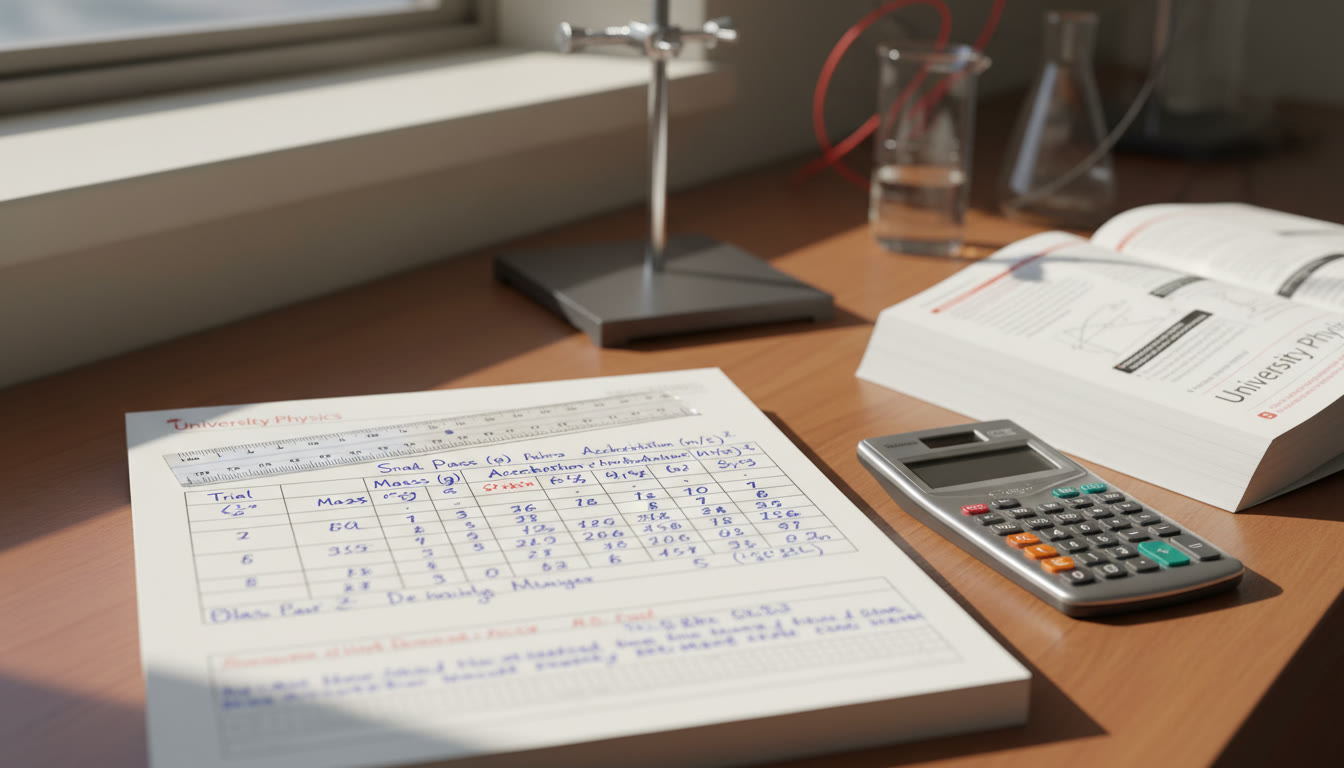
Why Data Tables and Error Bars Matter in AP Physics 2
Walk into any AP Physics 2 lab and you’ll quickly see that experimental skill is just as important as conceptual knowledge. Data tables and error bars are the language of experimental physics: they let you communicate measurements, quantify confidence, and compare theory to reality. A neat table without uncertainty is an incomplete story; a graph covered in error bars but lacking context is confusing. This guide walks you through creating clear data tables, estimating and propagating uncertainties, plotting and interpreting error bars, and using those tools to write stronger lab reports and earn the scores you want on College Board–style assessments.

Begin With Purpose: What Your Table Should Communicate
Every data table should answer three questions at a glance: What did you measure? How did you measure it (units and uncertainties)? And why does it matter (derived quantities or comparisons)? Keep these principles in mind:
- Clarity first: Use descriptive column headings, include units, and keep numerical precision consistent.
- Reproducibility: Record experimental conditions (temperature, instrument models, settings) nearby or in a note so others could repeat the experiment.
- Conciseness: Don’t cram everything into one table. If you have distinct sets of measurements (e.g., independent variable sweeps at different conditions), use separate tables or clearly partition the table.
Essential Columns for an AP Physics 2 Lab Table
At minimum, your table should include:
- Independent variable (label + units + uncertainty if applicable)
- Repeated raw measurements (if you took repeats)
- Mean values with standard deviation or standard error
- Derived quantities (calculated results with propagated uncertainties)
- Notes column for anomalies, outliers, or conditions
Designing a Table: A Practical Example
Imagine a simple AP Physics 2 lab: measuring the period of a simple pendulum for different lengths to investigate the small-angle approximation. Here’s a neat way to present data.
| Length L (m) | Trial 1 T (s) | Trial 2 T (s) | Trial 3 T (s) | Mean T (s) ± σT (s) | T^2 (s^2) ± propagated | Notes |
|---|---|---|---|---|---|---|
| 0.50 ± 0.001 | 1.42 | 1.43 | 1.41 | 1.42 ± 0.01 | 2.02 ± 0.03 | Small amplitude ~5° |
| 0.75 ± 0.001 | 1.74 | 1.73 | 1.75 | 1.74 ± 0.01 | 3.03 ± 0.04 | — |
| 1.00 ± 0.001 | 2.01 | 1.99 | 2.00 | 2.00 ± 0.01 | 4.00 ± 0.04 | — |
This table is concise, shows raw trials and summary statistics, includes instrument uncertainty (ruler precision), and carries the propagated uncertainty into the derived quantity T^2. In an AP lab report you would accompany this table with an explanation of how uncertainties were calculated and how they affect your conclusions.
Types of Uncertainty You’ll Encounter
Before you calculate anything, decide what kinds of uncertainty apply:
- Instrumental (systematic) uncertainty: The finite precision of rulers, timers, voltmeters—usually quoted as ± half the smallest division or given by the instrument specification.
- Random (statistical) uncertainty: Variation between repeated measurements due to uncontrolled fluctuations—a standard deviation quantifies this.
- Model or methodological uncertainties: Approximations in theory (e.g., assuming small-angle approximation) that might bias results.
Quick Recipes: Estimating Uncertainties
- For a single measurement from a ruler with 1 mm divisions, use ±0.001 m (or ±0.5 mm if you estimate between marks): that’s your instrument uncertainty.
- If you have multiple trials, compute the mean and the standard deviation σ. For reporting the uncertainty of the mean, use the standard error: σ/√N.
- If random and systematic uncertainties both apply, keep them separate and combine them at the end using the root-sum-square (RSS) method when appropriate.
Propagating Uncertainty: Keep the Math Simple and Transparent
When you calculate derived quantities (like T^2 or resistance R = V/I), you must propagate uncertainties so your final result has a meaningful error bar. Here are the most useful rules, explained plainly.
Basic Propagation Rules
- Addition/Subtraction: absolute uncertainties add. If Q = A ± B, then ΔQ = √(ΔA^2 + ΔB^2).
- Multiplication/Division: relative uncertainties add. If Q = A × B or Q = A / B, then (ΔQ / |Q|) = √((ΔA/A)^2 + (ΔB/B)^2).
- Powers: multiply relative uncertainty by the power. If Q = A^n, then ΔQ / |Q| = |n| × (ΔA / |A|).
Always show one worked example in your lab report. For instance, if mean T = 1.42 ± 0.01 s and we want T^2, then:
- Q = T^2 → relative uncertainty: 2 × (ΔT / T) = 2 × (0.01 / 1.42) ≈ 0.014
- Absolute uncertainty: ΔQ = Q × 0.014 ≈ 2.02 × 0.014 ≈ 0.03 s^2
Plotting Error Bars: Visualizing Confidence
A graph with error bars is often the clearest way to show whether your data supports a theoretical prediction. Error bars can represent standard deviation, standard error, or some confidence interval—just say which one. Here are practical tips for plotting and reading error bars in AP-style graphs:
- Label your axes and indicate units. Put a title or caption explaining what the error bars represent (±σ, ±standard error, or instrument uncertainty).
- Don’t clutter: If error bars overlap heavily among points, consider plotting mean with error bars and jittering raw trials slightly or use a separate inset for raw data.
- Fit with uncertainty: When fitting a line to data (e.g., T^2 vs L), include uncertainties in the fit routine if possible; otherwise, use the error bars to judge if the fit is consistent with data within errors.
Interpreting Overlap and Agreement
Two common misconceptions arise when seeing overlapping error bars. Overlap of error bars between two points does not automatically mean the points are statistically indistinguishable unless the error bars represent the same statistic and are large enough. For AP lab purposes, compare the predicted value to experimental points with their error bars: if the theory line passes through the error bar of a majority of points (or within combined uncertainty), your data and theory are consistent within experimental uncertainty.
Common Pitfalls and How to Avoid Them
- Too many significant figures: Don’t report uncertainties with more significant digits than the value justifies. If your mean is 1.42 ± 0.01, don’t write 1.423 ± 0.011.
- Combining unlike uncertainties: Keep systematic and random uncertainties distinguished in your analysis and state assumptions clearly.
- Neglecting units: Always include units in column headings and on axes—this is an easy point to lose on a lab rubric.
- Using a single trial: Whenever possible, take repeated trials. A single trial gives no measure of random error.
Writing the Lab Conclusion: Turn Numbers into Insight
In the conclusion section of an AP lab, your goal is to interpret results with uncertainty in mind. Don’t just say “the result matches theory.” Instead, follow this flow:
- Summarize the measured quantity and its uncertainty.
- Compare to the theoretical or accepted value, expressing the difference and whether it’s statistically significant given combined uncertainties.
- Assess possible sources of systematic error and how they would shift the result.
- Propose realistic improvements that would reduce uncertainty (better instrumentation, more repeats, control of environmental factors).
Example Conclusion Paragraph
“The measured dependence of T^2 on L produced a slope of 4.02 ± 0.07 s^2/m, which is consistent with the theoretical value of 4π^2/g = 4.03 s^2/m within experimental uncertainty. Instrumental uncertainty in length (±0.001 m) and timing jitter were the largest contributors; increasing the number of timing trials and using a photogate for period measurement would improve precision. Overall, our data supports the small-angle approximation for amplitudes near 5°, and deviations at larger amplitudes suggest nonlinear effects.”
Practical Tips for Lab Day Success
- Set up a clear data table template before you start taking measurements—this saves time and reduces transcription errors.
- Record raw data as you go; annotating anomalies immediately prevents confusion later.
- Use appropriate significant figures on calculators—round only at the end, but report with correct significant figures and uncertainty.
- Backup digital data (photos of analog displays or spreadsheets) so you can reference exact values if needed for grading or review.

How to Practice These Skills: Exercises and Mini-Labs
Deliberate practice is the fastest way to build confidence. Try these short exercises:
- Measure the same length with three different rulers (plastic, metal, laser) and create one table that compares means and instrument uncertainties.
- Time 20 oscillations of a pendulum five times, calculate mean period and standard error, and propagate uncertainty to T^2.
- Measure current and voltage for a resistor at several voltages; calculate R = V/I and propagate uncertainty from instrument precisions.
These small, repeated practices will make constructing tables and propagating errors second nature by the time the big lab write-up or the AP assessment arrives.
Using Tutoring and Tools Wisely
When you’re stuck on uncertainty propagation or need feedback on a lab report, tailored help can be a huge shortcut. Personalized tutoring—like the kind Sparkl offers—can provide 1-on-1 guidance, tailored study plans, and expert tutors who walk you through specific calculations and lab-writing strategies. They can point out subtle issues in your experimental design, recommend better measurement practices, and use AI-driven insights to identify consistent weaknesses so you improve faster.
Checklist Before You Submit Your AP Physics 2 Lab
Run through this checklist to make sure your lab report is complete and defensible:
- Are tables clearly labeled with units and uncertainties?
- Did you include raw trials and summary statistics (mean, σ, standard error)?
- Are propagated uncertainties shown for derived quantities?
- Do graphs have labeled axes, units, and clear error bars with a legend explaining what they represent?
- Is your conclusion quantitative (compare measured vs theoretical with uncertainties) and reflective (sources of error & improvements)?
- Did you include brief notes on measurement conditions and any data you discarded with justification?
Final Thoughts: Precision, Honesty, and Communication
AP Physics 2 lab success rests on three pillars: precise measurements, honest uncertainty analysis, and clear communication. Data tables are more than a place to dump numbers—they are the evidence you present to back up your scientific claims. Error bars are not admissions of failure; they are a scientific statement: this is how much we can reasonably trust our measurement. Master these skills, and your lab reports will not only score better but also reflect the way real scientists think and work.
And remember, when you need a focused push—whether a review of uncertainty propagation, help creating publication-quality tables, or practice problems tailored to your weak spots—personalized tutoring from services like Sparkl can turn confusion into clarity with targeted feedback and study plans. The effort you put into understanding and presenting uncertainty pays off on lab reports and on the AP assessment.
Quick Reference: Propagation Cheatsheet
| Operation | Quantity | Uncertainty Rule |
|---|---|---|
| Add/Subtract | Q = A ± B | ΔQ = √(ΔA^2 + ΔB^2) |
| Multiply/Divide | Q = A × B or A / B | ΔQ/|Q| = √((ΔA/A)^2 + (ΔB/B)^2) |
| Power | Q = A^n | ΔQ/|Q| = |n| × (ΔA/|A|) |
One Last Tip
Make neatness part of your scientific rigor. A readable table, a clear graph with labeled error bars, and an explanation that demonstrates you understand the role of uncertainty will carry more weight than a messy report with bigger numbers. Train yourself to be precise in both measurement and presentation—your future self (and your grader) will thank you.
Good luck—and enjoy the experiments!
Approach each lab as a story you’re telling with numbers: set the scene, gather evidence, analyze it honestly, and write a conclusion that ties it all together. With practice and the right support, data tables and error bars become not a chore, but a reliable toolkit for scientific thinking.


No Comments
Leave a comment Cancel