Why mastering lab skills matters for AP Chemistry (and beyond)
If you’re preparing for AP Chemistry, you already know the multiple-choice and free-response questions are just one part of the story. The ability to design experiments, collect accurate data, interpret results, and explain uncertainties is a huge part of what separates a good score from a great one. Calorimetry, spectrophotometry, and titration are the trio of classics you’ll see again and again—on lab practicals, in AP-style questions, and in real-world chemistry. This post walks through the ideas, the why and how, and practical strategies to make these techniques feel intuitive, not intimidating.
Roadmap: What we’ll cover
- Core principles: What each technique measures and why it’s useful.
- Step-by-step lab approach: Set up, measure, common pitfalls, and troubleshooting.
- Data and error analysis: How to look at your numbers like a scientist.
- Practice problems and real-world context: Quick examples you can try mentally or in the lab.
- Study strategy: How to practice efficiently, and when personalized tutoring can help.

Part 1 — Calorimetry: Measuring heat and making sense of energy
Fundamental idea
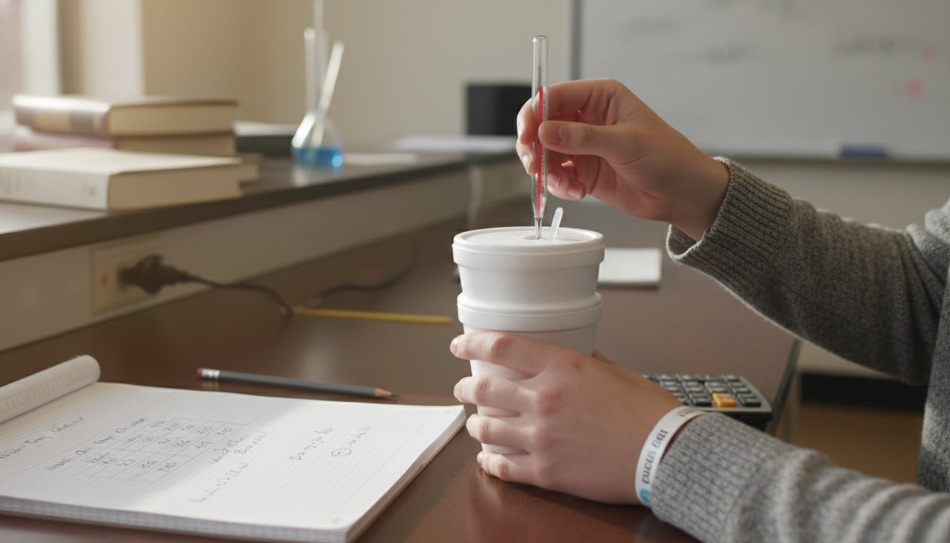
Calorimetry is the measurement of heat exchanged in a chemical or physical process. In AP contexts you’ll often see simple coffee-cup calorimeters (constant pressure) or bomb calorimeters (constant volume). The essential equation is q = m × c × ΔT (heat = mass × specific heat capacity × change in temperature). In reactions, remember that q(reaction) + q(calorimeter) + q(soln) = 0 if you treat the system and surroundings together.
Common setups and what they tell you
- Coffee-cup calorimeter: Great for solution reactions and neutralization—easy to assemble and ideal for labs where precision to ±0.1–0.5 °C is acceptable.
- Bomb calorimeter: Used for combustion, more sealed and accurate for complete combustion measurements.
- Calorimetry with phase changes: Track melting or freezing by monitoring temperature plateaus.
Practical step-by-step (coffee-cup style)
- Pre-lab: Calculate expected temperature changes from theoretical enthalpies to estimate detectability.
- Assemble: Insulate the cup, place a calibrated thermometer or temperature probe, and record the initial temperature once equilibrium is reached.
- Mix: Add reactant quickly, stir gently and continuously, and record temperature at regular short intervals (every 10–15 seconds initially).
- Analyze: Identify the maximum (or minimum) temperature after mixing, correct for heat capacity of calorimeter if known, and compute q using q = m × c × ΔT. Convert to molar quantities when reporting ΔH per mole.
- Post-lab: Consider heat losses to the environment—discuss sources of error and whether the calorimeter constant should be factored in.
Common pitfalls and troubleshooting
- Poor insulation — leads to systematic underestimation of |q|. Use a lid and minimize time between mixing and measurement.
- Inaccurate mass or concentration data — double-check balances and volumetric glassware.
- Delayed stirring or slow mixing — causes non-uniform temperatures; stir consistently.
- Thermometer calibration — if possible, verify with an ice bath (0 °C) and a known temperature point.
AP style tip
When writing free-response answers, always state assumptions (e.g., neglecting heat loss to surroundings) and include units. If asked for sign conventions, be explicit: exothermic reactions release heat so ΔH is negative; endothermic reactions absorb heat so ΔH is positive.
Part 2 — Spectrophotometry: Using light to measure concentration
Core principle
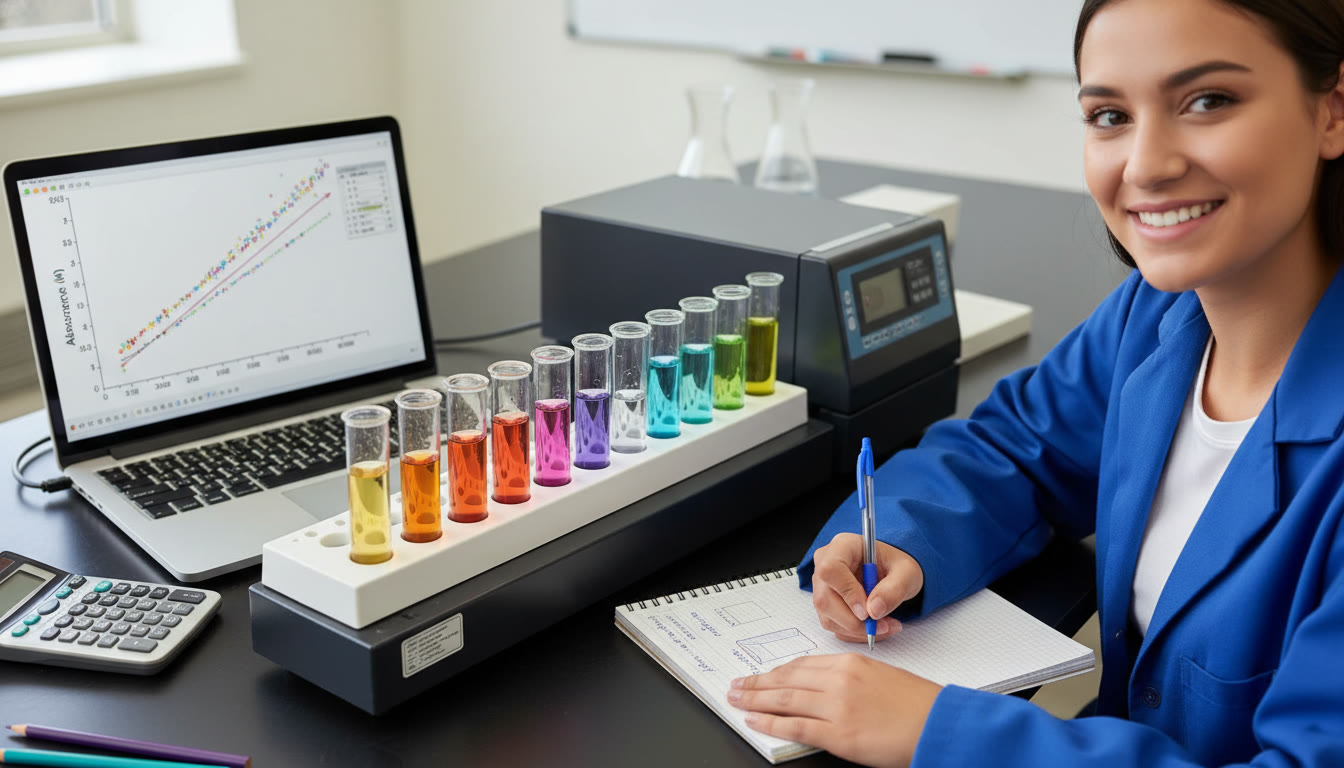
Spectrophotometry relies on the Beer-Lambert law: A = ε × l × c, where absorbance (A) is proportional to concentration (c). ε is the molar absorptivity and l is the path length (usually 1 cm). The instrument measures how much light at a chosen wavelength is absorbed by your solution—this lets you determine concentration precisely if you build a proper calibration curve.
Why it’s powerful for AP labs
Spectrophotometry connects quantitative analysis to molecular structure—specific chromophores absorb characteristic wavelengths. It’s ideal for kinetics (monitoring absorbance over time), equilibrium (using absorbance to find concentrations at equilibrium), and concentration determination via standard curves.
Step-by-step: getting accurate absorbance data
- Select wavelength: Scan or consult known λmax for your analyte; choose the wavelength where absorbance is highest (λmax) for sensitivity.
- Blank correctly: Zero the instrument with the exact solvent or matrix used in your samples (the blank removes background absorbance).
- Prepare standards: Make a series of standards that bracket the expected concentration range (e.g., 0.0, 0.1, 0.2, 0.5, 1.0 M or appropriate µM values). Use volumetric pipettes and flasks for accuracy.
- Measure: Rinse cuvettes, fill to consistent volume, and measure in the same orientation. Record replicate readings to check precision.
- Construct calibration curve: Plot absorbance vs concentration, perform linear regression (slope = ε × l), and use the fit to calculate unknown concentrations.
Errors to watch for
- Stray light and instrument limits: Very high absorbance (>1.5) is unreliable. Dilute samples into the linear range.
- Scattering and turbidity: Particulate matter scatters light and invalidates Beer-Lambert assumptions—filter if necessary.
- Non-linearity at high concentrations: Deviations from linearity can occur due to association, reabsorption, or instrument behavior.
Example: finding the concentration of a dye
Prepare standards at 0, 2, 4, 6, 8 µM, measure absorbance at λmax, and obtain a linear fit. If your unknown has absorbance 0.356 and the line is A = 0.045 × c (µM), the concentration is c = 0.356 / 0.045 ≈ 7.91 µM. Always report with appropriate sig figs and uncertainty from regression.
Part 3 — Titration: Precision at the buret tip
Basic concept
Titration is a controlled addition of a solution of known concentration (titrant) to a solution of unknown concentration until the reaction reaches an equivalence point. The equivalence point corresponds to stoichiometric completion; an indicator or pH meter reveals the endpoint (which should closely match equivalence if chosen well).
Common titrations in AP
- Acid–base titrations with indicators or pH meter (strong acid/strong base, weak acid/strong base, etc.).
- Redox titrations using a suitable oxidizing or reducing titrant.
- Complexometric titrations for metal ions (EDTA), less common but conceptually similar.
Practical approach and technique
- Standard solutions: Prepare or verify the concentration of titrant using primary standards when required.
- Buret technique: Fill without air bubbles, record initial volume to two decimal places, rinse the tip with titrant to avoid dilution errors.
- Endpoint detection: Choose an indicator with a color change near the expected equivalence pH, or use a pH meter/stacked end-point detection for precision.
- Perform multiple trials: At least two consistent titration results should be averaged; discard obvious outliers after checking technique.
Example calculation
If 25.00 mL of acid requires 18.65 mL of 0.1000 M NaOH to reach the endpoint, moles NaOH = 0.01865 L × 0.1000 mol/L = 0.001865 mol. If the reaction is 1:1, moles acid = moles NaOH, so [acid] = 0.001865 mol / 0.02500 L = 0.07460 M. Report with proper sig figs and include uncertainty from buret readings.
Common student mistakes
- Air bubbles in buret: causes erroneous volume readings—drain and re-zero carefully.
- Adding titrant too quickly near endpoint: overshooting is the most common source of error—use dropwise addition and swirl constantly.
- Incorrect indicator choice: color change window must match the expected pH at equivalence for clear endpoints.
Putting it together: Data, uncertainty, and how exam graders think
AP graders look for scientific reasoning, correct calculations, clear units, and honest discussion of error. When presenting results, do these things:
- Show raw data and computed values (temperatures, volumes, absorbances, masses).
- Include a sample calculation and then the final value with units and significant figures.
- State assumptions (e.g., neglect heat loss, assume 1.00 cm path length) and describe effects of systematic vs random errors.
- Estimate uncertainty: simple propagation (percent errors or range from repeated trials) demonstrates scientific maturity.
Simple error-propagation heuristics
If your result depends on multiplication/division (e.g., concentration calculation), sum relative uncertainties. For additions/subtractions (e.g., ΔT = Tfinal − Tinitial), add absolute uncertainties. You don’t need advanced math—clear, reasonable estimates earn credit.
Quick comparison table: When to use which technique
| Technique | Main Measurement | Typical Applications | Key Strength | Typical Uncertainty Sources |
|---|---|---|---|---|
| Calorimetry | Heat (q), ΔT | Reaction enthalpies, specific heat, phase-change energetics | Direct energy measurement | Heat loss to environment, calorimeter constant, thermometer error |
| Spectrophotometry | Absorbance (A) | Concentration determination, kinetics, equilibrium studies | High sensitivity, non-destructive | Stray light, turbidity, non-linearity at high concentration |
| Titration | Volume at endpoint | Concentration analysis, stoichiometry, equivalence point studies | Quantitative accuracy for molarity | Endpoint detection error, buret technique, standard solution errors |
Practice problems to deepen understanding
Try these as mini exercises (ideal for timed AP practice). Work them out by hand or in your lab notebook and remember to show assumptions and uncertainty estimates.
- Calorimetry: Mixing 50.0 g of water at 22.0 °C with 50.0 g of water at 62.0 °C—what is the final temperature? Now extend to a neutralization reaction releasing 25.0 kJ and compute the temperature change assuming perfect insulation and specific heat = 4.184 J/g·°C.
- Spectrophotometry: You build a calibration curve for an unknown dye. Standards give A = 0.100 at 2.0 µM and A = 0.500 at 10.0 µM. Is the Beer-Lambert law obeyed? Estimate ε × l and predict concentration for A = 0.350.
- Titration: A 20.00 mL sample of a diprotic acid requires 24.50 mL of 0.1000 M NaOH for complete neutralization. What is the concentration of the acid? (Hint: consider stoichiometry for a diprotic acid.)
How to practice efficiently (study plan)
Quality beats quantity. Focus practice sessions on weak spots and mix lab technique with conceptual review. A sample weekly rhythm might look like:
- Day 1 — Technique practice: one titration and one calorimetry calculation (write up clearly).
- Day 2 — Concept review: Beer-Lambert derivation and examples, equilibrium links.
- Day 3 — Timed AP-style questions mixing data analysis and short explanations.
- Day 4 — Reflection and targeted corrections: re-run calculations, practice uncertainties.
- Weekend — Mock lab write-up: prepare a full but concise lab report for one experiment and get feedback.
How Sparkl’s personalized tutoring can fit in
If you find specific techniques tricky, short targeted sessions with a tutor can speed up progress. Sparkl’s personalized tutoring offers 1-on-1 guidance, tailored study plans, and expert tutors who can walk through a titration setup, help interpret calorimetry data, or coach you through constructing and analyzing a spectrophotometric calibration curve. The right feedback—especially when paired with practice—turns confusion into clarity.
Real-world context: Why these skills matter outside AP
The same fundamentals appear across scientific careers: calorimetry in materials and food science, spectrophotometry in biochemistry and environmental monitoring, titration in pharmaceuticals and quality control. Knowing how to think about instrumentation, accuracy, and uncertainty prepares you not just for an exam but for real lab work.
Final checklist before lab practicals or the AP exam
- Know the formulas and when to use them: q = m·c·ΔT, A = ε·l·c, molarity calculations for titration.
- Understand instruments: how to zero a spectrophotometer, how to avoid air bubbles in a buret, how insulation affects calorimetry.
- Practice a few full write-ups: data table, sample calculation, final result, uncertainty discussion, and a brief sources-of-error paragraph.
- Simulate pressure: do a timed write-up to mimic AP free-response timing and grading expectations.
Parting thought: Be curious, not just correct
Lab work rewards curiosity. When you get a strange number, don’t hide it—ask why. Might your calorimeter be absorbing heat? Could your indicator shift color too early? Was your spectrophotometer saturating? This mindset—paired with clear technique and thoughtful analysis—will serve you well on the AP exam and in any scientific endeavor. If you want targeted practice, consider short sessions with a tutor to sharpen technique and build confidence; many students find that a few focused lessons turn uncertainty into consistent performance.
Ready to practice?
Pick one technique and build a short plan: perform or simulate one experiment, record data carefully, write a clear analysis, and then repeat focusing on the biggest source of error you found. Repeat this cycle and you’ll move from tentative to confident. Good luck—measure carefully, think critically, and enjoy the discovery.


No Comments
Leave a comment Cancel